2.4. Symmetry Breaking

Introducing mass to gauge bosons will break the U(1) local gauge symmetry.

But wait, why preserving U(1) symmetry?

1. But wait, why do we need to preserve U(1) symmetry?
2. We introduce mass to bosons regardless of the breaking of U(1) symmetry.
3. Such a mass term will lead to infinity in e-e scattering loop. (By counting the orders of moment, we know this is not finite.)
4. Introduce cut-off to momentum.
5. Still have infinity in higher order loop diagrams.
6. Introduce infinite numbers of cut-off for the infinite infinities of infinite higher order loop diagrams.
7. WTF.

So we can not just simply introduce the mass term.

2.4.1. Spontaneous Breaking of Gauge Symmetry

We can not simply write a mass term in the Lagrangian. However, mass is simply an interaction term quadratic in the field, e.g. \(-m^2\phi^2\). Geometrically speaking, we need a upward opening quadratic potential of the field, i.e., Fig. 2.1.

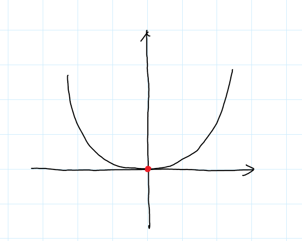
Fig. 2.1 To have mass we need a potential with parabola shape at least around the minimium which is the vacuum. Another requirement is that the potential should be bounded.

The point is, since we are talking about the perturbation around the minima, we can also construct a potential with more complicated shape but is has quadratic term around the minina, e.g., Fig. 2.2.

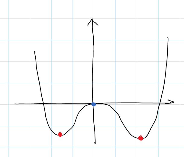
Fig. 2.2 This potential also have a parabola shape around the minima.

2.4.1.1. Spontaneous Breaking Global Gauge Symmetry

Mathematically the simplest Lagrangian for a real scalar field that could possibly have a mass that we can think of is

\[\mathcal L = \frac{1}{2}\partial_\mu \phi \partial^\mu \phi - \frac{1}{2} \mu^2 \phi^2 - \frac{1}{4}\lambda \phi^4,\]

where we set \(\mu^2 < 0\) and \(\lambda > 0\).

Notice that we have global gauge symmetry holds. By intuition we expect the field to have a quadratic shape around the minima since this is a quartic potential. Indeed we Taylor expand the potential around the right minimaium \(\phi_0\),and define a new field around the minimium \(\eta(x) = \phi(x) - \phi_0\). The Lagrangian becomes

\[\mathcal L ' = \frac{1}{2} \partial_\mu \eta \partial^\mu \eta - \lambda \phi_0^2 \eta^2 + \text{higher order terms} + \text{constant},\]

where we spot the quadratic term \(- \lambda \phi_0^2 \eta^2\) so that mass of the field \(\eta\) around its vacuum (minimium) can be defined as \(m^2 \equiv \lambda \phi_0^2\).

The two Lagrangians describes the samething around the minimium point \(\phi_0\). We notice that the global gauge invariance is broken for field \(\eta\).

What is broken?

Both Lagrangian \(\mathcal L\) and \(\mathcal L'\) are invariant under the global gauge transformation of field \(\phi\). But they are all changed under a gauge transformation of field \(\eta\).

What does that mean?

Since our particle physics are always dealing with small amount of particles, the physics is described by a field near the minimium potential point, which can be called vacuum of the field. When we are doing experiments near the vacuum, we do not see the big picture that the whole potential is quartic.

That is to say, we are talking about a field :math:`eta` that varying around a minimium potential point. What we see is a small parabola (quadratic terms) with some corrections (higher order terms). Any potential that can give us a parabola like potential at its minimium will possibly work.

The same trick can be done for complex fields. The Lagrangian we are interested in is

\[\mathcal L = \partial_\mu \phi^* \partial^\mu \phi - \mu^2 \phi^* \phi - \lambda (\phi^* \phi)^2,\]

where we also have \(\mu^2 < 0\) and \(\lambda > 0\). The potential is a Mexican hat, c.f. Fig. 2.3.

Fig. 2.3 Density plot of the quartic potential. Darker color means smaller potential while brighter color means larger potential. The ring is where the potential minimium is located.

Mathematica code for the density plot

range = 1.5; DensityPlot[Log[1000 (1/4 (x^2 + y^2)^2 - 1/2 (x^2 + y^2) + 1/4)], {x, -range, range}, {y, -range, range}, Frame -> False, PlotRange -> Full, ColorFunction -> GrayLevel(“SunsetColors”), PerformanceGoal -> “Quality”, ColorFunctionScaling -> True, PlotPoints -> 300, Axes -> True, AxesLabel -> {“Re[[Phi]]”, “Im[[Phi]]”}, Ticks -> None, ImageSize -> Large]

Since we have two degrees of freedom, we can look at two directions. The direction that circles the ring is the direction that the potential has no change, while the perturbation in the radial direction needs to climb on and off potentials. The potential in the radial direction has a quadratic term around minima. The radial direction perturbation generates mass, however the circular direction perturbation doesn’t generate mass. The massless boson is Goldstone boson, which becomes a problem because we get a massless mode of the particle.

Similar picture can be established for three component fields, which has a potential minimium on a 3D spherical surface. The perturbation around that minimium needs three degrees of freedom, thus generating 2 massless Goldstone bosons and one massive boson and one massive boson in the perturbation of radial direction.

2.4.2. Spontaneous Breaking of Local Gauge Symmetry

To keep the local gauge invariance, we write the Lagrangian as

\[\mathrm D_\mu \phi^* \mathrm D^\mu \phi - \frac{1}{4} F_{\mu\nu}F^{\mu\nu},\]

where covariant derivative is \(\mathrm D_\mu = \partial_\mu - i eA_{\mu}\). Perform the trick of quartic potential, the Lagrangian becomes

\[\mathcal L = \mathrm D_\mu \phi^* \mathrm D^\mu \phi -\mu^2 \phi^*\phi - \lambda (\phi^* \phi)^2 - \frac{1}{4} F_{\mu\nu}F^{\mu\nu}.\]

Why a negative sign for the kinetic term of gauge field \(-\frac{1}{4} F_{\mu\nu}F^{\mu\nu}\)?

Quick and simple answer:

Check the components that contains the time derivative of the field \(A_\mu\).

Local gauge transformation

\[\begin{split}\phi \to & e^{i\alpha(x)}\phi , \\ A_\mu \to & A_\mu + \frac{1}{e} \partial_\mu \alpha.\end{split}\]

To work out the perturbation theory, we take the old school treatment,

\[\phi = \frac{1}{\sqrt{2}}(\phi_0 + \eta + i\xi ).\]

The expanded Lagrangian is

\[\mathcal L' = \frac{1}{2} \partial_\mu \eta \partial^\mu \eta + \frac{1}{2} \partial_\mu \xi \partial^\mu \xi - \phi_0^2 \lambda \eta^2 + \frac{1}{2} e^2 \phi_0^2 A_\mu A^\mu - e \phi_0 A_\mu \partial^\mu \xi - \frac{1}{4}F_{\mu\nu} F^{\mu\nu} + \text{other terms}.\]

We are super happy to locate the terms \(- \phi_0^2 \lambda \eta^2\) and \(\frac{1}{2} e^2 \phi_0^2 A_\mu A^\mu\) since they give mass to \(\eta\) field and \(A_\mu\) gauge field.

Problems

However, we still have a massless Goldstone boson \(m_\xi=0\).

Meanwhile, we notice that the term \(- e \phi_0 A_\mu \partial^\mu \xi\) is weird because we have a direct transformation from one field to another!

HINT

Or maybe not? We do not expect such direct tranformation. But maybe they are actually the SAME field! By interpreting the \(\xi\) field as part of the gauge field can eliminate the massless Goldstone boson.

To support such conjecture, we need to choose a different set of real field instead of the original \(\eta\), \(\xi\), and \(A_\mu\). We have been using Cartesian coordinates since the very beginning of this trick. But polar coordinates are better for spherically symmetric potential. So we rewrite the field as

\[\begin{split}\phi =& \frac{1}{\sqrt{2}} (\phi_0 + h(x)) e^{i \theta(x)/\phi_0}, \\ A_\mu' = A_\mu + \frac{1}{e\phi_0} \partial_\mu \theta,\end{split}\]

where \(h\), \(\theta\) are real and \(\phi_0\) is where the minimium potential is reached.

A miracle happens immediately,

\[\mathcal L' = \frac{1}{2} \partial_\mu h \partial^\mu h - \lambda \phi_0^2 h^2 + \frac{1}{2} e^2\phi_0^2 A'_\mu A'^\mu + \frac{1}{2} e^2 A'_\mu A'^\mu h^2 - \lambda \phi_0 h^3 - \frac{1}{4} \lambda h^4 + \phi_0 e^2 A'_\mu A'^\mu h - \frac{1}{4} F_{\mu\nu} F^{\mu\nu}.\]

The field \(\theta\) is gone. Meanwhile the two real fields \(h\) and \(A_\mu\) gain mass.

What is the magic?

The magic is that the massless Goldstone boson by field \(\xi\) becomes part of the gauge field \(A_\mu\).

Mathematically, we notice that the two expansion are related to each other under the condition of perturbation in both fields

\[\frac{1}{\sqrt{2}} (\phi_0 + h) e^{i\theta/\phi_0} = \frac{1}{\sqrt{2}} (\phi_0 + h) (1 + i \frac{\theta}{\phi_0}) = \frac{1}{\sqrt{2}} (\phi_0 + h + i \theta + i \frac{h\theta}{\phi_0}),\]

where the last term \(i \frac{h\theta}{\phi_0}\) is higher order in the perturbation fields so we drop it. Field \(h\) corresponds to \(\eta\) while field \(\theta\) corresponds to \(\xi\).

However, the difference is that here we do not need to perturb the field \(\theta\) since it’s gone in the Lagragian. And it should NOT be in there in principle. The perturbation method using \(\eta\) and \(\xi\) introduced a spurious field.

2.4.3. References and Notes

1. Halzen & Martin